Inference Is Where the Money Goes

Everyone talks about training. The GPU clusters, the weeks of compute, the eye-watering budgets. It makes for a good story, and it is the part of the process that gets a press release.

But training happens once. Inference happens every single time a user hits enter. Multiply that by every user, every message, every day the product is alive, and the arithmetic stops being close: the majority of what you spend on a model, you spend running it, not making it.

I have been working through DeepLearning.AI’s Fast & Efficient LLM Inference course, built with Red Hat and taught by Cedric Clyburn, and writing up what I learned as I go. This first part is the ground floor: why serving efficiently is worth caring about, what actually happens inside the model when it produces a token, and where every byte of your GPU memory ends up. The later parts get hands-on with quantization, vLLM, and benchmarking.

The problem changed

In early 2023 there were essentially no competitive open-source models. Today there are thousands of them on Hugging Face, from basically every organization that trains models — OpenAI included.

So the question flipped. It used to be can I get a good model? Now it is can I run this model efficiently?

Which raises the obvious follow-up: why run it yourself at all, instead of calling somebody’s API? Four reasons come up over and over:

• Cost. Instead of paying per token, you match model size to task difficulty. Not every request needs your largest model.
• Security. The data never leaves your environment. In healthcare or financial services that is frequently not a preference but a requirement.
• Control. You decide when a model upgrades or gets deprecated. No rate limits, no third-party outage taking your product down with it.
• Customization. You can fine-tune for your domain, which buys you accuracy and cost control at the same time.

None of that is free. You are trading somebody else’s operational problem for your own, and the rest of this article is about what that problem looks like.

Two numbers decide whether your deployment is good

Like any production system, an LLM deployment needs measurable targets — service level objectives. There are two dimensions worth tracking, and you need both.

Accuracy, because a model that is wrong is not useful. A model that hallucinates, or answers off-brand, fails regardless of how fast it is. The threshold depends entirely on your use case, and the way you check it before deploying is the model card. Model cards for optimized variants publish a row per standardized benchmark — MMLU for general knowledge, GSM8K for math, and so on — alongside a recovery column showing how much of the original model’s accuracy the optimized version retains. When you see something like 99.88% average recovery on a compressed model, that number is what you hold your accuracy SLO against.

Inference performance, because a model nobody wants to wait for is also not useful. Three latency metrics matter:

• Time to first token (TTFT) — how long the user stares at nothing before anything appears.
• Inter-token latency (ITL) — the average gap between consecutive output tokens, excluding the first. This is what “smooth” or “choppy” generation actually means.
• Request latency — total time, end to end.

And alongside latency, throughput: the average number of output tokens generated per second across all requests. Latency is the single user’s experience; throughput is whether your system survives production scale.

Small gaps in either dimension become big problems later. To be useful, a deployed model has to be both fast enough and accurate enough.

The hardware math

Here is where it gets concrete. GPU memory has to hold two things: the model weights, which occupy a fixed amount of space whether you are serving one user or a hundred, and the KV cache, which is working memory that grows with every token and every active request.

These two behave nothing alike, and that difference is the whole game.

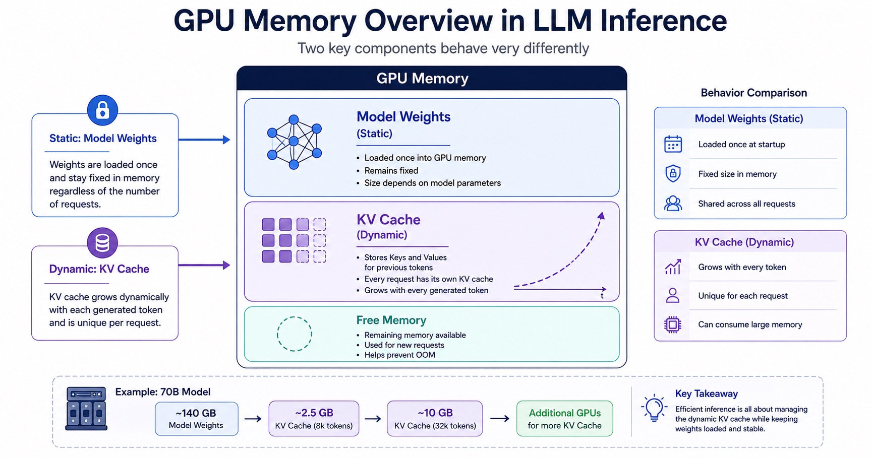
Take Llama 3 at 70 billion parameters. At the precision it shipped in, a parameter is roughly two bytes, so the weights alone need about 140 GB. That means at minimum two 80 GB GPUs just to load the thing.

Nobody deploys it that way. The standard production unit for a 70B-class model is four 80 GB GPUs — 320 GB total, which leaves about 180 GB for everything else.

That “everything else” is almost entirely KV cache. For Llama 3 70B, a single long-context request at 32,000 tokens needs roughly 10 GB of KV cache by itself. So with 180 GB of headroom, you can serve about 18 long-context users in parallel.

Except you can’t, not by default. A naive serving setup with no memory optimization manages that space so badly that the same hardware serves two or three.

Eighteen versus three, on identical GPUs. That gap is the entire subject of this course.

Two places to optimize

The techniques for closing that gap fall into two categories, and they are genuinely different in kind.

Model optimizations happen to the model itself, before it is ever deployed. Quantization, sparsification. The goal is to reduce the memory footprint and the compute required while preserving as much accuracy as you can. You do this once, you get an artifact, you ship the artifact.

Inference optimizations happen at runtime, inside the serving engine. Continuous batching, prefix caching, PagedAttention. These do not change the model at all — they change how efficiently you run it.

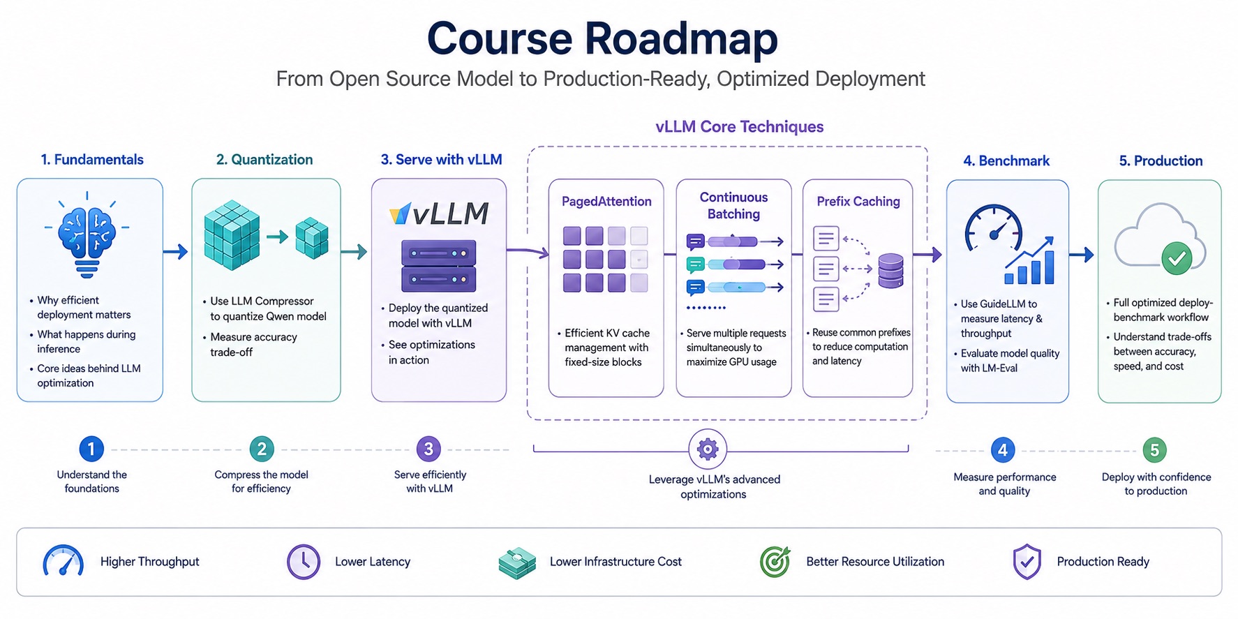
Both matter, and they compose. But there is a constraint underneath all of it that never goes away:

Performance, accuracy, cost. Most deployments get to pick two.

Real-time latency means your users are not waiting around, but high throughput usually wants more compute. Accuracy earns trust, but bigger models with better evals cost more. And you need infrastructure spend to stay sane — except aggressive model optimization can eat into accuracy. The right tooling pushes those limits further out than you would expect, but it does not repeal the tradeoff.

To put rough numbers on the shape of it: a naive deployment of a 70B model at full precision, processing one request at a time, can run into hundreds of thousands or millions of dollars a month at real user volume. Add continuous batching and proper KV cache management via PagedAttention, and throughput improvement alone takes roughly an order of magnitude off the bill. Then add a quantized model on the same server — smaller footprint, faster weight loading, better use of the GPU’s hardware — and it drops again.

That is the destination. Now the fundamentals, because none of those techniques make sense until you know what they are optimizing.

What inference actually is

When you send a prompt — a question, a code suggestion, a document to summarize, or these days an agent doing it on your behalf — what happens under the hood is inference: using a trained model to generate a response.

Running that in production takes three pieces stacked together:

• The model at the top: the file holding billions of learned parameters.
• The inference server in the middle: software like vLLM that loads the model, manages incoming requests, and implements every optimization in this article.
• The hardware accelerator at the bottom: usually a GPU, doing the numerical heavy lifting.

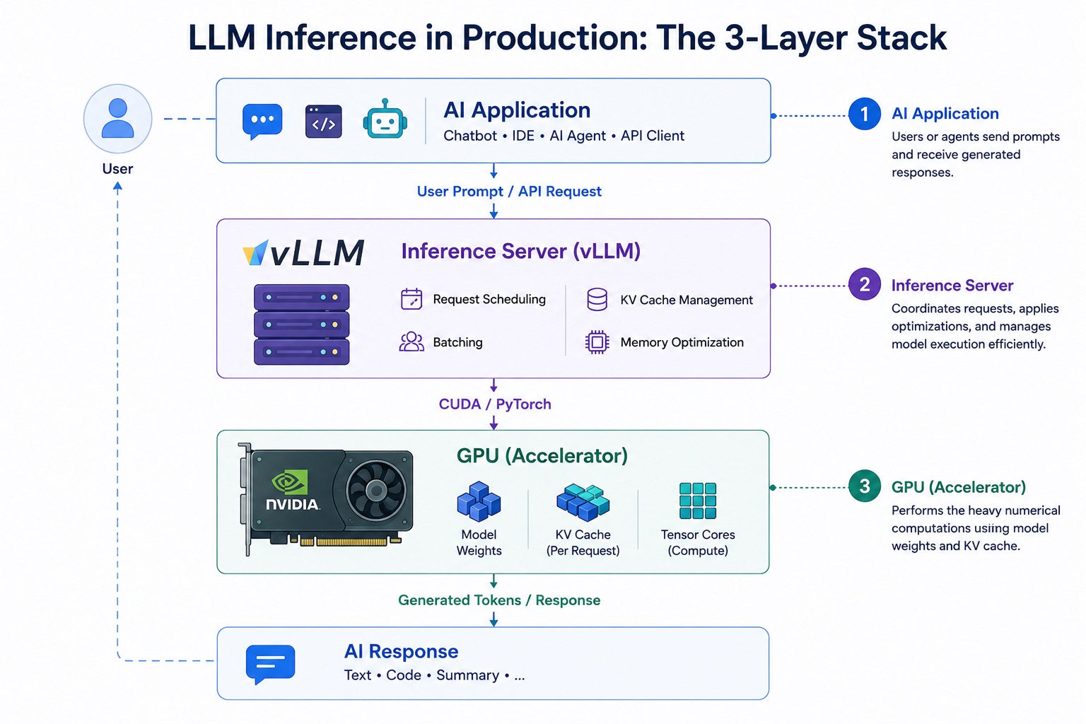
You can skip the middle layer. Loading a model straight onto a GPU with PyTorch works fine — for a notebook, or one user. The moment you need to serve many users at once, the inference server stops being optional. It is the piece that makes the GPU usable at production scale.

One token at a time

LLMs do not produce a sentence. They produce a token, then another token, where a token is roughly a word or a piece of one.

The loop is simple enough to trace by hand. You send The quick brown. The model processes it and predicts the next token: fox. That token gets appended, so the input is now The quick brown fox, and the model runs again, predicting jumps. Append, run again, over. This continues until the model emits a special end-of-sequence token meaning it is done.

This is autoregressive generation, and the important property is that each new token depends on every token before it — including the ones the model just wrote itself.

Which means every token in a response requires a full pass through the model. A 500-token answer is 500 forward passes.

Inside one forward pass

So what is a forward pass?

The model converts each input token into a vector of numbers — a token embedding. Those embeddings flow through a stack of transformer layers. Each layer has two parts: a self-attention block, where tokens exchange information with each other, and a feed-forward network, which processes each token’s representation further. That pair repeats N times, stacked.

After the final layer, the output goes through the LM head, which turns the model’s internal representation into a score for every possible next token. Highest score wins — fox, at 90% probability. Then that token gets appended to the input, and the whole stack runs again.

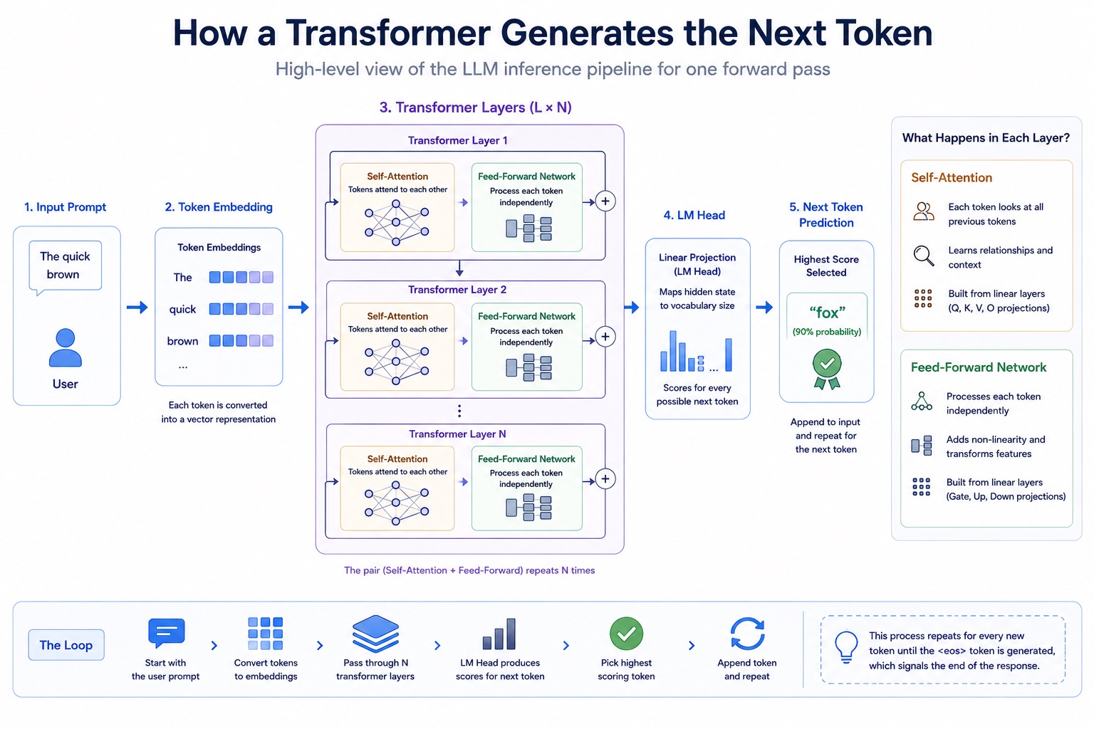
Zoom into one transformer layer and both blocks turn out to be built from the same primitive: linear layers. A linear layer is a matrix multiplication. Take a vector, multiply by a weight matrix, get a new vector. That is the whole operation.

It is also where almost all of the model’s parameters live, and where almost all of the computation happens.

• Self-attention holds four linear layers: the Q, K, V, and O projections. This is where tokens look at each other to work out how they relate.
• The feed-forward network holds three: gate, up, and down projections. These process each token independently, with no interaction between tokens.

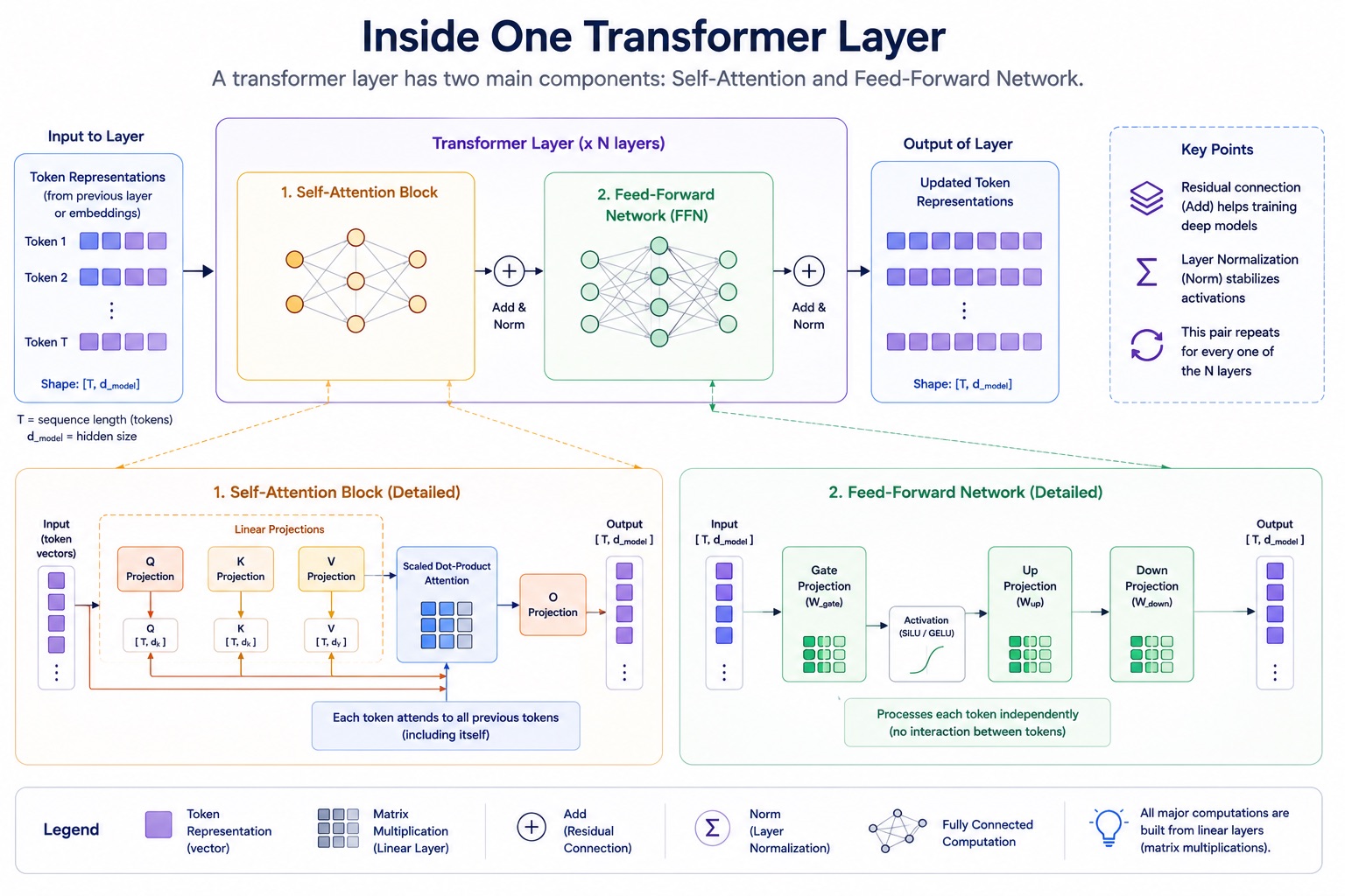
These weight matrices are learned once during training and then never change. Everything the model does — understanding tokens, relating them, predicting the next one — comes down to these linear layers doing matrix multiplications, over and over, across N transformer blocks, for every single token generated.

Attention, concretely

Self-attention is where each token pays attention to the others. When the model reads The quick brown fox, attention is the mechanism that lets fox know it is connected to quick — that the fox is the thing that is quick.

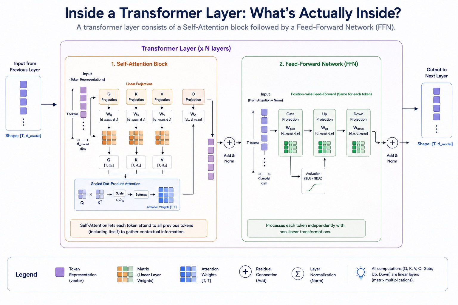
To do that, three vectors get computed for the token in question. Each comes from passing the token’s current representation through a separate linear layer:

• Q, the query: what do I want to know from the context?
• K, the key: here is my label, and the kind of information I hold.
• V, the value: if my label matches, here is my actual content.

The token’s “current representation” is its input embedding if this is the first transformer layer, or the output of the previous layer otherwise.

Computing attention for fox then goes like this. Take its query Q and compare it against the key of every token so far, including itself, using a dot product. High dot product means this token is relevant to me; low means it is not. For a four-token sequence that gives four raw scores.

Divide those scores by the square root of the key dimension to keep the numbers numerically stable, then push them through a softmax so they become weights that sum to one. Say token 2 comes out highest at 0.52 — the model thinks token 2 matters most to token 4.

Finally, take a weighted sum of all the value vectors using those weights. The result is one vector, now enriched with context from the rest of the sequence. It passes through o_proj, the fourth linear layer, and that is the attention block’s output.

The observation that gives you the KV cache

Look closely at what that computation needed.

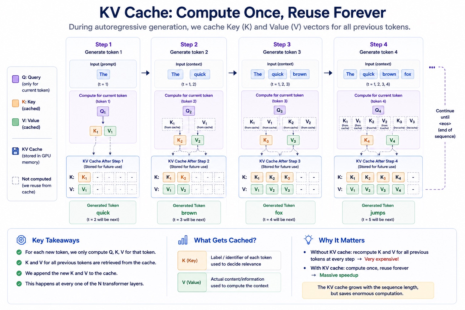
To generate a new token, you need the keys and values of every previous token in the sequence. But the query is only needed for the current token. Q is per-step. K and V are the entire history.

That asymmetry is the whole idea.

Walk it forward. The model generates token 4, fox, computing Q4, K4, V4. Attention uses Q4 together with the keys and values of all previous tokens. Now it generates token 5, jumps — and for that it needs a new query Q5, plus a new K5 and V5. But K and V for tokens 1 through 4 have not changed. Nothing about them could have changed. Recomputing them would be pure waste.

So you don’t. After computing K and V for a token, you save them in GPU memory. On every subsequent step you compute K and V only for the new token and append them to the cache; attention pulls the rest from storage.

That is the KV cache. And because it happens at every one of the N layers, the savings multiply by N.

How big it gets

Per token, you store a key and a value vector at every layer. One detail matters enormously here and is easy to read past.

Each layer runs attention in parallel across many heads, so the model can capture several kinds of relationship at once. Llama 3 70B has 64 of them. But it does not store 64 sets of keys and values — it stores eight.

That is grouped-query attention (GQA): groups of eight query heads share a single key/value head. The queries stay diverse; the cache does not multiply. This is not an architectural footnote — it is the single biggest reason the numbers below are survivable at all.

The count that goes into the size formula is therefore the number of KV heads, not attention heads. Per token:

2 × num_layers × num_kv_heads × head_dim × dtype_bytes

The 2 is because you store both K and V. For Llama 3 70B: 80 layers, 8 KV heads, head dimension 128, and two bytes per number at its release precision.

2 × 80 × 8 × 128 × 2 = 327,680 bytes ≈ 320 KB per token

Per token. Scale that to context lengths people actually deploy at:

| Context length | What it is | KV cache | | --- | --- | --- | | 2,000 tokens | a typical chat turn | ~640 MB | | 8,000 tokens | standard production tier | ~2.5 GB | | 32,000 tokens | a long document or codebase | ~10 GB | | 128,000 tokens | Llama 3’s maximum | ~40 GB |

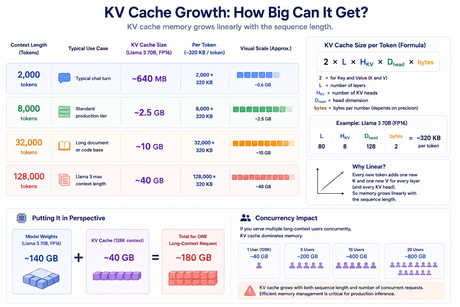
Worth pausing on how much GQA is doing for you here. Store all 64 heads instead of 8 and the per-token figure becomes roughly 2.5 MB, which turns that last row into ~320 GB — more than twice the model’s own weights, for one conversation. Grouped-query attention is what makes long context economically possible at all.

Sit with the numbers as they stand, though. The model’s own weights are about 140 GB. A single max-context request needs 40 GB of KV cache on top — nearly a third of the model’s entire size, for one user’s conversation.

And it is per request. Serve ten concurrent long-context users and you need over 400 GB of KV cache alone, before the model.

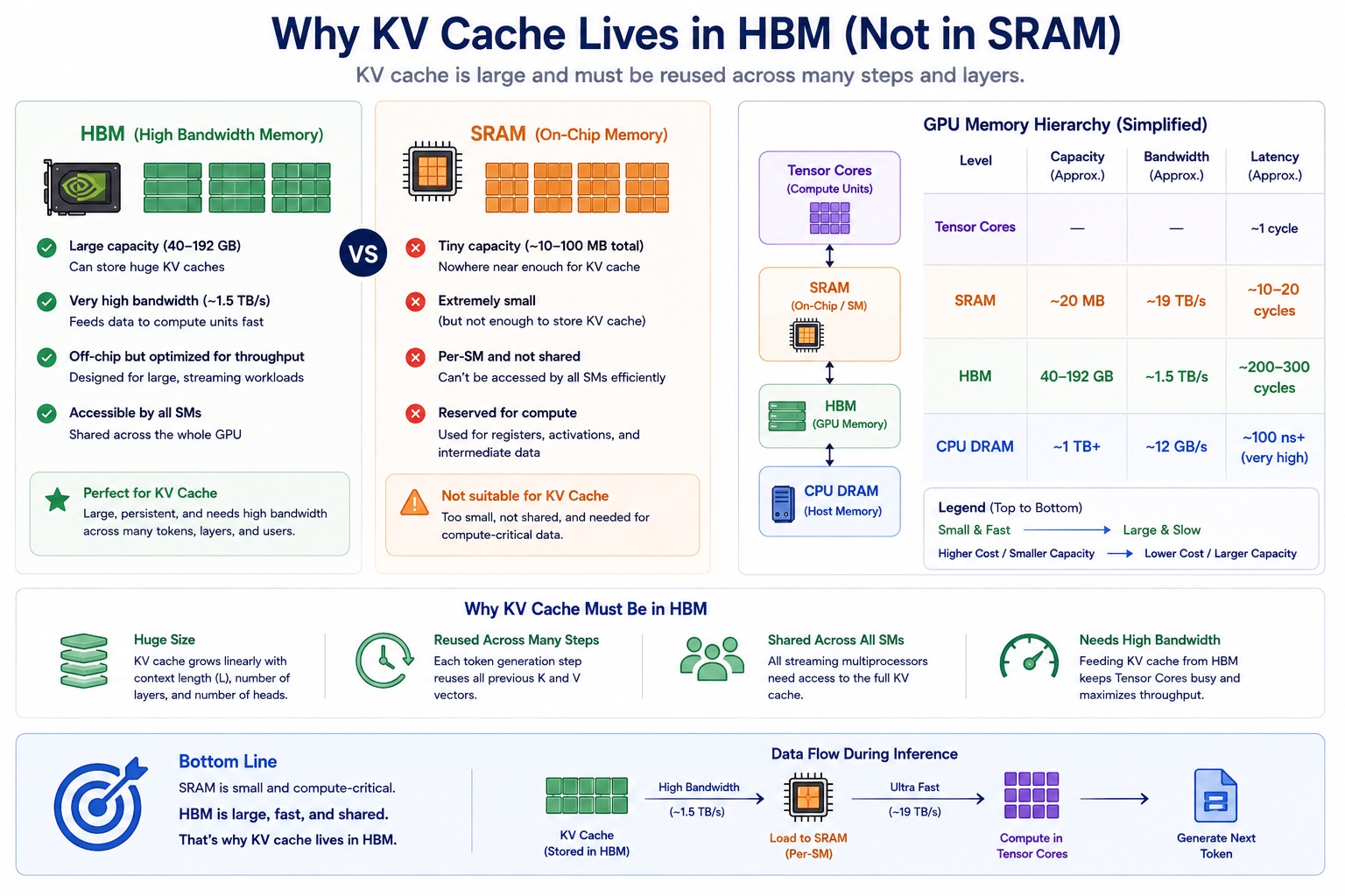
This is why the KV cache, not the weights, is the dominant memory concern in modern LLM inference. It lives in GPU memory, it grows linearly with both sequence length and concurrent requests, and managing it efficiently is the single biggest job a production inference server has.

Where the tensors actually live

You now know the two things sitting in memory during inference. Worth zooming out to look at the memory system they live in.

A quick vocabulary note first. So far I have used vector, matrix, and intermediate values fairly loosely. The general term for any multi-dimensional array of numbers is a tensor. A single number is a zero-dimensional tensor, a vector is one-dimensional, a matrix is two-dimensional. Q, K, V, the KV cache, and the model’s weights are all tensors. From here on, “data moving through the model” just means tensors.

A GPU has three tiers of memory, and they differ dramatically in both size and speed.

CPU DRAM sits at the bottom — the host machine’s main memory. A GPU is not a standalone computer; it plugs into a host with its own CPU and RAM. That host memory varies enormously, from 16 GB in a laptop to a terabyte or more in a datacenter server. Whatever the size, it is far from the GPU, and moving data across that boundary is slow compared to anything happening on the card itself.

HBM — high bandwidth memory — sits in the middle. This is what people mean when they say “GPU memory” or VRAM. It is on the GPU card, close to the compute units. Smaller than host memory, much faster.

SRAM sits at the top: on-chip memory right next to the GPU’s compute units. Those units are tensor cores, specialized hardware that performs matrix multiplications extremely fast — which is exactly what every linear layer in the model needs. Tensor cores read their inputs from SRAM, do the math, write results back. SRAM is tiny and extraordinarily fast, and its whole job is keeping the tensor cores fed.

Concrete numbers, using the NVIDIA A100:

| Tier | Size | Bandwidth | | --- | --- | --- | | SRAM | ~20 MB | ~19 TB/s | | HBM | 40 GB | ~1.5 TB/s | | Host ↔ GPU transfer | (host DRAM) | ~12 GB/s |

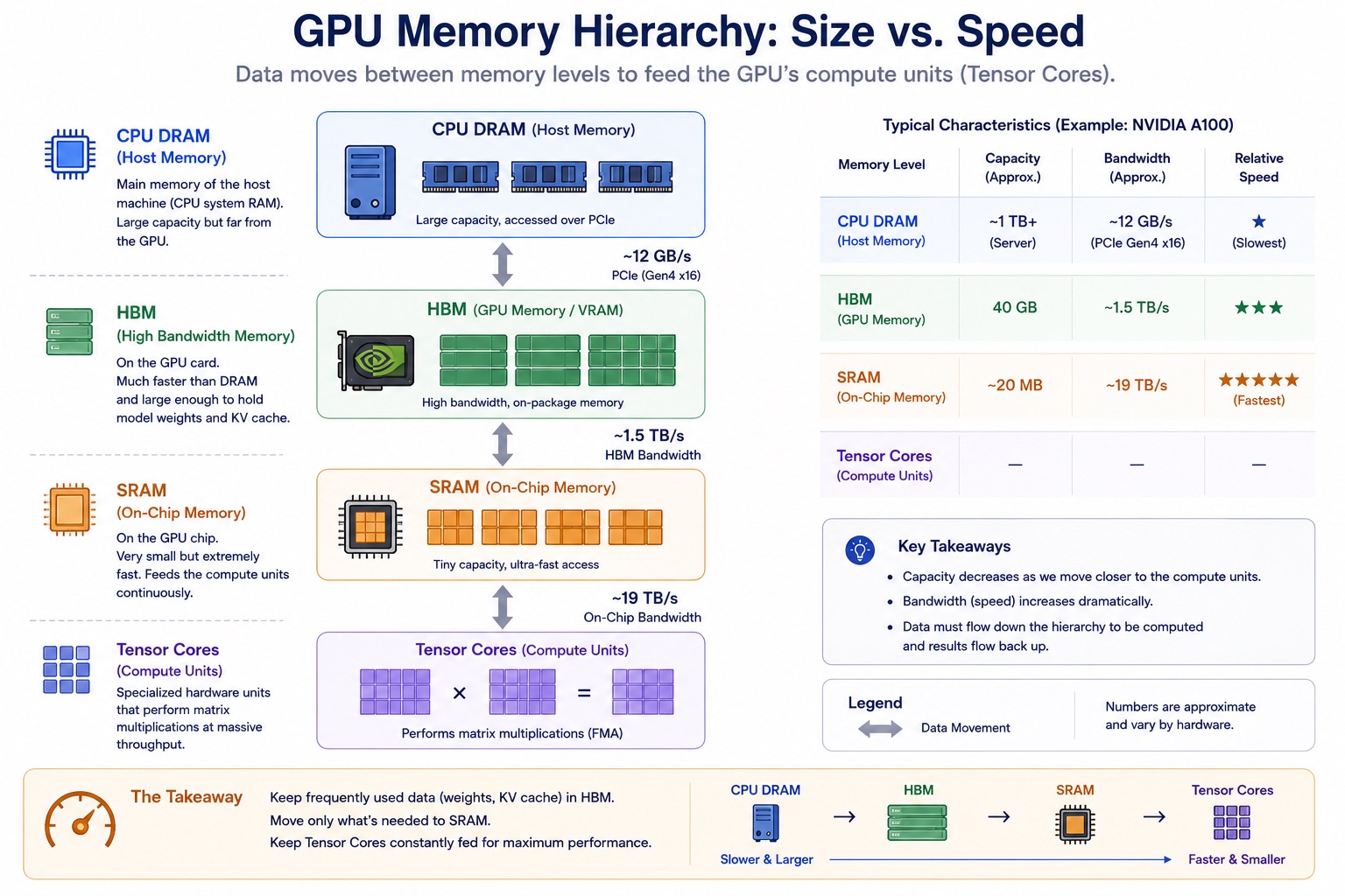
The tradeoff is clean and it is the same tradeoff at every level of every memory hierarchy ever built: the closer memory sits to the compute units, the faster it is, and the less of it there is.

So where does inference actually put things?

Model weights load from disk or host DRAM into HBM once, at startup, and stay there for the lifetime of the server. The KV cache also lives in HBM, growing as each request processes more tokens. During every forward pass, small chunks of the weights and the KV cache get pulled from HBM into SRAM so the tensor cores can work on them. This happens over and over — for every linear layer, at every one of the N transformer layers, for every token generated.

There are also transient tensors produced at each step: the query vector for the current token, the attention output, the intermediate outputs of each feed-forward layer. Note that the step’s K and V are not in that list — those get appended to the KV cache and stay. The genuinely transient ones are allocated in HBM alongside everything else, streamed through SRAM in tiles as the tensor cores consume them, and freed once the step is done.

That detail is worth being precise about, because it is exactly what fused kernels attack. FlashAttention is the canonical example: its entire value is keeping some of these intermediates resident in SRAM rather than writing them out to HBM and reading them back a moment later.

The two things that bound you

Which leaves two levers, and only two, on how fast inference can possibly go:

1. How fast data moves from HBM into SRAM.
2. How fast the tensor cores compute on it once it arrives.

Every optimization in the rest of this series comes back to that. Move less data, move it more efficiently, or manage the memory better. Quantization shrinks what has to move. PagedAttention manages where the KV cache sits. Continuous batching makes each trip carry more useful work.

So let’s start with the first one.

The gap keeps widening

Models have been getting more capable, and they have been getting much larger at the same time. More parameters means more memory, more compute, more cost.

Plot model size over time on a log axis and the trend is brutal: the original Transformer in 2017 at 50 million parameters, today’s frontier models in the hundreds of billions, some past a trillion. Model sizes have roughly doubled every year.

GPU memory has not. It has grown, but nothing close to that rate. So the gap between what models can do and what hardware can actually run keeps opening up.

That mismatch creates four concrete problems:

• Infrastructure. Bigger models mean more accelerators, often spread across multiple nodes, and that gets expensive fast.
• User experience. More parameters means slower responses, lower throughput, and less room left in the KV cache for long context.
• Energy. Every extra GPU draws power. At scale that is a real environmental cost, not a rounding error.
• Obsolescence risk. You invest in infrastructure sized for a model that gets superseded six months later.

Compression is how you close that gap.

Quantization: store fewer bits

The idea is almost embarrassingly simple. Think of a weight as π. You could store 3.14159265… or you could store 3.14. The second one is less precise and much smaller.

Most LLMs ship at BF16 — 16 bits per number. Quantization converts those numbers into lower-bit formats: FP8, INT8, INT4. Fewer bits per number, smaller model overall.

A quick note on the naming, because it looks like alphabet soup until someone spells it out:

• FP is floating point — numbers with decimals, like 3.14.
• BF is brain floating point. BF16 is a 16-bit format developed by Google with a wider range than FP16, which makes it more numerically stable for large models. That stability is why it became the default release format.
• INT is integer — whole numbers, like 3 or −127.

The thing worth internalizing is that range and precision are separate knobs. FP32 covers a huge range with fine-grained precision, meaning tiny gaps between representable values. BF16 covers the same range as FP32 but with bigger gaps in between — that is the trade Google made. Move down to FP16 and INT8 and the range shrinks too, while the gaps keep growing.

You are always trading precision for size.

Quantization can be applied to two different things: the weights, which are the model’s learned parameters, and the activations, which are the intermediate values computed during a forward pass. That distinction matters more than it sounds like it should, and I will come back to it.

There is also sparsification, which attacks the problem from a different angle: zero out the weights that contribute least to the model’s predictions so they can be skipped entirely at inference time. A common approach is 2:4 sparsity, where two out of every four values in a weight tensor are set to zero, cutting both memory and computation.

What this buys you, counted in GPUs

Abstractions are unconvincing. Here is Llama 4 Scout at 109 billion parameters.

| Format | Bits/param | Weights | GPUs (80 GB) | | --- | --- | --- | --- | | BF16 (as shipped) | 16 | ~220 GB | 3 | | INT8 / FP8 | 8 | ~109 GB | 2 | | INT4 / FP4 | 4 | ~55 GB | 1 |

BF16 is two bytes per parameter, so 109B × 2 ≈ 220 GB, which needs at least three 80 GB GPUs. Drop to 8 bits — one byte — and 109B × 1 ≈ 109 GB. Half the memory, two GPUs. Go to 4 bits and you are at roughly 55 GB: a 75% reduction, and the whole model fits on one GPU.

Same model. Three GPUs to one. That is the infrastructure bill changing shape.

Where in the model this actually happens

From the earlier sections: a model is a stack of transformer blocks, each containing a self-attention block with four linear layers and a feed-forward network with three.

Those linear layers are where quantization is focused. Not everywhere — there are other components, notably the embedding layer at the start and the LM head at the end, and those are typically excluded from quantization to preserve accuracy.

Why target the linear layers specifically? Two reasons, and they are the same two reasons that show up everywhere in this article: most of the time during a forward pass is spent inside them, because that is where the main matrix multiplications happen, and the bulk of the model’s weights live there. Highest impact per unit of risk.

Inside a linear layer there are two things you can quantize:

• The weights — the learned matrix.
• The input activations — the tensor that gets multiplied by those weights.

Input activations are simpler than the name suggests. Anything that flows into a linear layer and gets multiplied by its weights is an input activation. Inside attention, that could be the tensor representation of fox flowing into the Q, K, and V projections. It could equally be the weighted-sum output flowing into o_proj. They are just tensors moving through the network, getting multiplied by weights along the way.

Two wins, and they are not the same win

This is the part I found genuinely clarifying, because quantization does not just save memory — its two effects map directly onto the memory hierarchy from earlier.

Quantized weights buy you lower latency, on the data-movement side. Every forward pass, the GPU pulls weights from HBM into SRAM so the tensor cores can work. If those weights are 8 bits instead of 16, there is literally half as much data to move. It moves faster. Inference gets faster.

Quantized activations buy you higher throughput, on the compute side. Tensor cores can perform more operations per second when the numbers are in lower-precision formats. Modern GPUs — Hopper, Ada Lovelace, and newer — have dedicated FP8 tensor cores; on older Ampere hardware, INT8 tensor cores play the same role.

So weight quantization speeds up the moving. Activation quantization speeds up the math. Quantizing both is what unlocks the full speedup, and this gives you a real choice when compressing a model:

| Scheme | What is quantized | At inference time | What you win | | --- | --- | --- | --- | | W8A16 (weight-only) | weights only, e.g. to INT8 | weights load from HBM compressed, then get dequantized back to BF16 just before the multiply | less data moved; no tensor core speedup | | W8A8 | weights and activations, e.g. to INT8 or FP8 | the math itself runs on low-precision tensor cores | less data moved and more ops/second |

With weight-only quantization the tensor cores still do their math in higher precision, so the win is purely on data movement. W8A8 reduces the memory cost and the compute cost.

In practice that compounds into five things: fewer GPUs needed, lower deployment cost, decreased latency, higher throughput and longer context (because memory freed from weights goes back to the KV cache), and lower energy consumption.

What it looks like on real traffic

Benchmarks in the abstract are easy to dismiss, so here is a realistic workload — RAG, where the model answers a question using documents pulled from a knowledge base.

The input is 1,024 tokens, broken into three pieces: 50 tokens of system prompt (“answer using the provided context”), 20 tokens for the user’s actual question, and 900 tokens of retrieved context — the documents holding the answer. The output is about 128 tokens.

Lots of context going in, a moderate response coming out. Exactly the shape where quantization should pay off, because there is a lot of data to move and a lot of compute to do.

Results, comparing an FP16 baseline against FP8 with weights and activations quantized, on Llama 3 70B running on two H100s:

| Metric | FP16 baseline | FP8 (W8A8) | | --- | --- | --- | | Throughput (input tokens/sec, at load) | plateaus ~158 | climbs to ~474 | | Time to first token (at high load) | over 30,000 ms | ~4,800 ms |

Over 3× the throughput on identical hardware. And the latency number is the one that should get your attention: under heavy load the FP16 baseline’s TTFT explodes past 30 seconds — a user staring at nothing for half a minute — while FP8 stays comparatively flat, peaking around 4.8 seconds. Roughly a 6–7× reduction in latency at high load, from a change that costs you no hardware at all.

But does the model get worse?

This is the obvious question. You are throwing away precision. Something must break.

The honest answer is: when quantization is done correctly, essentially no. But done correctly is carrying real weight in that sentence.

Naive quantization — blindly rounding every number down to fewer bits — does hurt the model. What works in practice are calibrated techniques like GPTQ, AWQ, and SmoothQuant. Instead of rounding blindly, these run a small representative dataset through the model to work out which weights and values matter most, and protect those during quantization.

The evidence comes from evaluating quantized models on three reasoning benchmarks: AIME 2024 (30 expert-level competition math problems), MATH-500 (a curated set of 500 challenging problems), and GPQA-Diamond (expert-validated science questions). The metric is average pass@1 — the percentage of problems the model gets right on its first attempt, averaged across all three. Higher is better.

Across model sizes from Llama-8B up to Qwen-32B, four precision formats were compared: BF16 as the baseline, FP W8A8, INT W8A8, and INT W4A16 — the most aggressive scheme, with 4-bit weights.

The high-level result is that the bars are essentially the same height everywhere. Zoom into Qwen-14B for specifics:

| Format | Average pass@1 | | --- | --- | | BF16 (original) | 73.6 | | INT W4A16 (4-bit weights) | 72.8 | | FP W8A8 | 74.3 |

The most aggressive scheme on the chart — four-bit weights, a 4× shrink — costs less than a single point.

And the FP W8A8 row scores higher than the original. Not because quantization made the model smarter. The difference is small enough to be run-to-run variation. But it makes the point cleanly: at 8-bit floating point, having halved the model, there is in some cases no meaningful accuracy loss at all.

Done correctly, quantization gives you the speed and memory wins without giving up model quality.

Next: how GPTQ and AWQ actually pull that off, and compressing a model by hand.